Implementing SingleOptimizable

This tutorial will lead you step-by-step through the implementation of an example minimization problem. It touches on the usage of the Common Optimization Interfaces (cernml.coi) in particular as well as the problems of testing, packaging and machine communication in general.

If you want to look up specific parts, feel free to skip to them. Each section should be self-contained enough to answer at least several “How do I do X again?” questions.

The Problem

The first step (as always) is to set up your general project structure, declare dependencies, etc. We assume that you’ve already done so. If not, the previous tutorial will walk you through these steps.

Interactions with the Machine

It’s time to actually start implementing our problem! We start by adding a new module to our package:

# coi_example/__init__.py
"""An example for how to use the cernml-coi package."""

from .env import AwakeElectronBeamSteering

__version__ = "0.0.1.dev0"

and importing a few things we will need later (and only those things):

# coi_example/env.py
"""Implementation of the AWAKE e-beam steering problem."""

import time
import typing as t

import gymnasium as gym
import numpy as np
from cernml import coi
from pyjapc import PyJapc

Not much to see yet, but this will change quickly. Let’s write a class that either creates a JAPC object or accepts one from the outside. The latter is necessary for embedding your problem into applications that manage JAPC centrally.

# coi_example/env.py (cont.)
class AwakeElectronBeamSteering:
    """Awake electron-beam steering optimization problem."""

    def __init__(self, japc: t.Optional[PyJapc] = None) -> None:
        if japc is None:
            japc = PyJapc("", incaAcceleratorName="AWAKE")
        self.japc = japc

Note that it’s not required to use JAPC. It is perfectly valid to define an optimization problem that does not use a PyJapc object and does not accept a japc parameter in its constructor. This makes sense if e.g. you write simulation of an optimization problem and don’t actually talk to the machine.

In any case, with this class in place, we can write methods to communicate with the corrector magnets:

# coi_example/env.py (cont.)
    CORRECTOR_ADDRS = (
        "logical.RCIBH.430029/K",
        "logical.RCIBH.430040/K",
        "logical.RCIBH.430104/K",
        "logical.RCIBH.430130/K",
        "logical.RCIBH.430204/K",
        "logical.RCIBH.430309/K",
        "logical.RCIBH.412344/K",
        "logical.RCIBH.412345/K",
        "logical.RCIBH.412347/K",
        "logical.RCIBH.412349/K",
    )

    def _send_corrector_values(self, values: t.Container[float]) -> None:
        if len(values) != len(self.CORRECTOR_ADDRS):
            raise ValueError(
                f"expected {len(self.CORRECTOR_ADDRS)} corrector values, "
                f"got {len(values)}"
            )
        for addr, value in zip(self.CORRECTOR_ADDRS, values):
            self.japc.setParam(addr, value)
        time.sleep(1)

    def _recv_corrector_values(self) -> np.ndarray:
        return np.array(self.japc.getParam(self.CORRECTOR_ADDRS))

Notice that we define their addresses in a class-level attribute and use JAPC to send and receive values. Notice also that in the setting method, we introduce a small delay to ensure that the values have arrived at the machine before we continue.

Great! Let’s do the same for the BPM readings. Because JAPC sends us back a lot of information about each BPM, we have to write a small helper function to extract the parts we are interested in:

# coi_example/env.py (cont.)
    BPM_ADDRS = (
        "TT43.BPM.430028/Acquisition",
        "TT43.BPM.430039/Acquisition",
        "TT43.BPM.430103/Acquisition",
        "TT43.BPM.430129/Acquisition",
        "TT43.BPM.430203/Acquisition",
        "TT43.BPM.430308/Acquisition",
        "TT41.BPM.412343/Acquisition",
        "TT41.BPM.412345/Acquisition",
        "TT41.BPM.412347/Acquisition",
        "TT41.BPM.412349/Acquisition",
        "TT41.BPM.412351/Acquisition",
    )

    def _recv_bpm_readings(self) -> np.ndarray:
        values = self.japc.getParam(self.BPM_ADDRS)
        return np.array([_extract_bpm_reading(value) for value in values])


def _extract_bpm_reading(bpm_reading: dict) -> float:
    pos_ok: np.ndarray = bpm_reading["posOK"]
    if not any(pos_ok):
        return 0.0
    hor_pos: np.ndarray = bpm_reading["horPos"][pos_ok]
    return np.mean(hor_pos)

Note that the helper function _extract_bpm_reading() is not part of the class because it doesn’t need to access any attributes of it.

The Interface

With this, we have all the primitive operations in place to start implementing the optimization-problem interface. We kick this off by editing our class definition: Instead of being its own independent class, it now subclasses the SingleOptimizable interface:

# coi_example/env.py

class AwakeElectronBeamSteering(coi.SingleOptimizable):
    """Awake electron-beam steering optimization problem."""

    # Rest same as before …

The interface requires the following information from us:

• Distribution metadata

• The Optimization Space

• The Initial Point x₀

• The Objective Function

and the following ones are optional (i.e. we’ll get to them later):

• Constraints

• Custom Rendering Output

The Metadata

Let’s start with the boring one, the metadata: Every optimization problem must declare a minimal amount of information about itself so that the host application that runs it knows how to handle it. We insert the metadata class attribute at the top of the class, for maximum visibility:

# coi_example/env.py

class AwakeElectronBeamSteering(coi.SingleOptimizable):
    """Awake electron-beam steering optimization problem."""

    metadata = {
        "render_modes": [],
        "cern.machine": coi.Machine.AWAKE,
        "cern.japc": True,
    }

    # Rest same as before …

Metadata is basically a free-form dictionary. You’re free to put in your own information if you think you need to. However, some keys are standardized and have conventional meaning. The full list is given elsewhere, but the important parts are:

"render_modes"

This must be present and it must be a collection of strings. We’ll get to the details further down, but this declares the ways in which a user can visualize your problem. Because this list is empty right now, it means our problem can’t be visualized at all. (We’ll change this later.)

"cern.machine"

This declares the CERN accelerator that your problem belongs to. If this is set to None or is missing, we assume that this problem isn’t related to any accelerator at all.

"cern.japc"

If this is present and True, it means that our problem requires JAPC access. In such a case, our __init__() method must accept a keyword argument japc (which it already does).

The Optimization Space

The optimization_space is a definition of how many parameters we are optimizing (the degrees of freedom) and what their valid domains are. We define it in our __init__() method, which now looks like this:

# coi_example/env.py
    def __init__(self, japc: PyJapc = None) -> None:
        if japc is None:
            japc = PyJapc(selector="", incaAcceleratorName="AWAKE")
        self.japc = japc
        ndim = len(self.CORRECTOR_ADDRS)
        self.optimization_space = gym.spaces.Box(-1.0, 1.0, shape=(ndim,))

For now, the space must always be a box, its shape must always be a one-tuple with the number of degrees of freedom, and the bounds are always −1 and +1. These restrictions may be lifted in the future.

The Initial Point x₀

Every optimization procedure needs an initial point from where to start optimization. The method get_initial_params() provides this point to the host application.

While we are free to supply any initial point that we want (even a random one!), we decide to measure the corrector values at instantiation and return those. This gives the host the possibility to always return to a known-good state: By simply using those initial settings without doing any optimization!

We add two lines to the end of __init__():

# coi_example/env.py
    def __init__(self, japc: PyJapc = None) -> None:
        if japc is None:
            japc = PyJapc(selector="", incaAcceleratorName="AWAKE")
        self.japc = japc
        ndim = len(self.CORRECTOR_ADDRS)
        self.optimization_space = gym.spaces.Box(-1.0, 1.0, shape=(ndim,))
        self.initial_kicks = self._recv_corrector_values()
        self.corrector_scale = 0.1

and implement the method:

# coi_example/env.py (cont.)
    def get_initial_params(self) -> np.ndarray:
        return self.initial_kicks.copy() / self.corrector_scale

Note the self.corrector_scale: Our optimization space is normalized to the range from −1 to 1, but the actual corrector values may not. For now, the interface requires us to do this normalization manually. In the future, this restriction may be lifted in a backwards-compatible manner.

The Objective Function

Finally, it’s time to write the core of the class: The cost function that an optimizer will have to minimize. Note that the interface always assumes a minimizer. If you have, for whatever reason, a maximizing optimizer you will have to write a small adapter function that negates the result of compute_single_objective().

With all the work we’ve already done, writing this method is straight-forward. Again, we stay mindful of the fact that params is normalized to the range from −1 to 1:

# coi_example/env.py (cont.)
    def compute_single_objective(self, params: np.ndarray) -> float:
        self._send_corrector_values(params * self.corrector_scale)
        pos = self._recv_bpm_readings()
        rms = np.sqrt(np.mean(pos ** 2))
        return rms

Class Registration

Once all this is done, we already can use this class in an interactive session. However, to use it inside a host application, we must make one more step. We need to register it so that the host application can find it without having to scour our entire package.

Registration is done with a single line at the global scope:

class AwakeElectronBeamSteering(coi.SingleOptimizable):
    # Same as before …
    ...


coi.register(
    "AwakeElectronBeamSteering-v0",
    entry_point=AwakeElectronBeamSteering,
)

This line runs once our module is imported and ensures that our problem can be found under the given name via the COI registry.

Optimization Test Run

With all of these pieces in place, we can finally run our optimization problem. Fire up an interactive interpreter session, load an optimizer and our class, and everything runs on its own:

>>> # Instantiate our class. By virtue of importing coi_example, our
>>> # class has appeared in the registry and can be found by name.
>>> import coi_example
>>> from cernml import coi
>>> awake = coi.make("AwakeElectronBeamSteering-v0")
>>> # Run minimization. This part is completely generic and works with
>>> # every imaginable subclass of SingleOptimizable.
>>> from scipy.optimize import Bounds, minimize
>>> opt_space = awake.optimization_space
>>> minimize(
...     awake.compute_single_objective,
...     x0=awake.get_initial_params(),
...     bounds=Bounds(opt_space.low, opt_space.high),
... )

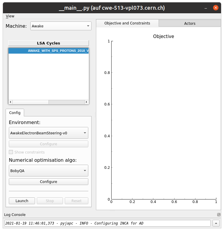
We can also pass our environment into the Generic Optimization Frontend and Framework and run it in there:

$ acc-py app run acc-app-optimisation ./coi_example/

If we choose AWAKE as a machine and expand the environment selector, we should see our class. Clicking on it should at least instantiate it without errors. Unfortunately, we won’t be able to run it, as this would require access to AWAKE itself. If we were able to, this class would already be usable.

Constraints

Some optimization algorithms (such as COBYLA) have a concept of constraints, i.e. linear or nonlinear functions whose value must be kept within certain bounds during optimization. The API allows specifying such constraints for your optimization problem, if it makes sense. To do this, you have to use LinearConstraint or NonlinearConstraint from the Scipy package:

from cernml import coi
from scipy.optimize import NonlinearConstraint

class UnrelatedProblem(coi.SingleOptimizable):
    def __init__(self):
        self.constraints = [
            NonlinearConstraint(self._constrain_beam_intensity, 1e10, np.inf),
        ]
        ...

    def compute_single_objective(self, params):
        self._apply_params(params)
        return self._calculate_loss()

    def _constrain_beam_intensity(self, params):
        self._apply_params(params)
        return self._calculate_beam_intensity()

    ...

Warning

Not all optimizers support constraints! When writing your optimization problem, you must assume and expect that the optimizer will ignore your constraints. Do not use constraints to implement safety-critical checks and limits. Use optimization_space and, in case of emergencies, raise an exception inside compute_single_objective().

Custom Rendering Output

The Generic Optimization Frontend and Framework (GeOFF) already provides some plotting out of the box; concretely, this is the loss over time, the corrector settings over time, and any possible [constraints](#constraints). For most optimization problems, this is all they need and no more code needs to be written.

Nonetheless, the COI provide way to implement fully flexible and customized plotting facilities for your optimization problem. This is provided through the render() method, which has been taken over from the Gymnasium interface for reinforcement learning.

The Mechanics

The way it works is that every time the render() method is called on a problem, it should visualize its current state in some way. (In our case, the current state is the latest readings from the BPMs.) The way in which this should happen is the render mode. It is passed to your __init__() method as a string and you should keep it around as a render_mode attribute.

A few Standard Render Modes have been defined by Gymnasium and the COI package. The ones that interest us are:

"human"

The default render mode. The problem should present itself on the current display or terminal and return None.

"matplotlib_figures"

Create one or more matplotlib.figure.Figure objects and use them for visualization. Return a list of Figure objects.

Implementing rendering involves these three steps:

1. Declare the supported render modes in the "render_modes" metadata.

2. Accept a parameter render_mode in your __init__() with None as a default value.

3. Override the Problem.render() method.

Rendering for Humans

We start out by modifying a few lines of code we’ve already written. We add imports of Matplotlib:

# coi_example/env.py
import gymnasium as gym
import numpy as np
from cernml import coi
from matplotlib import pyplot
from matplotlib.axes import Axes
from pyjapc import PyJapc

We add the render mode "human" to the list of supported render modes:

# coi_example/env.py (cont.)
    metadata = {
        "render_modes": ["human"],
        "cern.machine": coi.Machine.AWAKE,
        "cern.japc": True,
    }

And we now accept the render_mode parameter. We pass it to our super method in SingleOptimizable because that will automatically check it for correctness and set it as a self.render_mode attribute:

# coi_example/env.py (cont.)
    def __init__(self, japc: pyjapc = none, render_mode: str | none = none) -> none:
        super().__init__(render_mode)
        if japc is none:
            japc = pyjapc(selector="", incaacceleratorname="awake")
        self.japc = japc
        ndim = len(self.corrector_addrs)
        self.optimization_space = gym.spaces.box(-1.0, 1.0, shape=(ndim,))
        self.initial_kicks = self._recv_corrector_values()
        self.corrector_scale = 0.1

We will also add a new attribute self.latest_readings whose value we will visualize in render():

# coi_example/env.py (cont.)
    def __init__(self, japc: pyjapc = none, render_mode: str | none = none) -> none:
        super().__init__(render_mode)
        if japc is none:
            japc = pyjapc(selector="", incaacceleratorname="awake")
        self.japc = japc
        ndim = len(self.corrector_addrs)
        self.optimization_space = gym.spaces.box(-1.0, 1.0, shape=(ndim,))
        self.initial_kicks = self._recv_corrector_values()
        self.latest_readings = self._recv_bpm_readings()
        self.corrector_scale = 0.1

    def compute_single_objective(self, params: np.ndarray) -> float:
        self._send_corrector_values(params * self.corrector_scale)
        pos = self._recv_bpm_readings()
        rms = np.sqrt(np.mean(pos ** 2))
        self.latest_readings = self._recv_bpm_readings()
        rms = np.sqrt(np.mean(self.latest_readings ** 2))
        return rms

With this out of the way, we can start implementing render():

# coi_example/env.py (cont.)
    def render(self) -> t.Any:
        if self.render_mode == "human":
            _, axes = pyplot.subplots()
            self.update_axes(axes)
            pyplot.show()
            return None
        return super().render()

    def update_axes(self, axes: Axes) -> None:
        """Render this problem into the given axes."""
        axes.clear()
        axes.plot(self.latest_readings, "|-")
        axes.set_xlabel("BPM")
        axes.set_ylabel("Beam position (mm)")

Our plan is to follow a specific pattern in this implementation: A series of statements of the form if self.render_mode == ... followed by a call to super().render(). Each if handles one of the defined render modes, and if the render mode is unknown, we delegate to the base implementation, which raises a NotImplementedError. This prevents us from silently swallowing typos in the render mode.

Another notable choice is that we have put the rendering into a separate method. Not only does this keep the code cleaner, it will also be useful later, when we also implement the "matplotlib_figures" render mode.

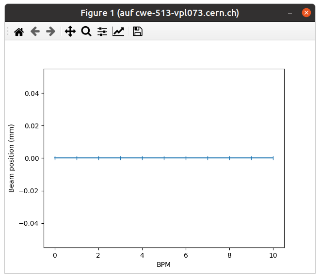
To test our implementation, we can simply call the method in an interactive Python session:

>>> from pyjapc import PyJapc
>>> from coi_example import AwakeElectronBeamSteering
>>> # Create our own PyJapc and pass `noSet` so that we don't
>>> # accidentally interfere with the accelerator operations.
>>> japc = PyJapc("", noSet=True, incaAcceleratorName="AWAKE")
>>> env = AwakeElectronBeamSteering(japc, render_mode="human")
>>> env.render()

Unfortunately, unless AWAKE itself is operational, this will likely only produce a flat line. Nonetheless, it shows that our method does what it is supposed to do.

Rendering for the App

The human render mode is useful for quick debugging, but it would not work when embedding our optimization problem into a GUI. Most crucially, pyplot.show() is a blocking function – it waits indefinitely and only returns once the user closes the window. If we called it inside a GUI, the entire application would freeze indefinitely!

Hence, we need another render mode, one that leaves the caller of render() in full control. At the same time, we don’t want to give up the convenience of the Matplotlib API. This is exactly what "matplotlib_figures" is for.

Note

The Pyplot API is so convenient because it manages a lot of global state for us: it tracks the set of open windows, the current figure*, the current axes into which all plotting goes, etc.

When embedding our class into a GUI app, this state management is already being done by the app. If we now used Pyplot on top of the GUI, the two would likely get into conflict with each other about who manages what.

For this reason, it is crucial for "matplotlib_figures" that no pyplot function is used. We will have to use the underlying Matplotlib API instead. Luckily, our helper method already does so!

To implement the new render mode, once again, we need to make a few changes in the previous code. We add another import:

# coi_example/env.py
import gymnasium as gym
import numpy as np
from cernml import coi
from matplotlib import pyplot
from matplotlib.axes import Axes
from matplotlib.figure import Figure
from pyjapc import PyJapc

We add the new render mode:

# coi_example/env.py (cont.)
    metadata = {
        "render_modes": ["human", "matplotlib_figures"],
        "cern.machine": coi.Machine.AWAKE,
        "cern.japc": True,
    }

And we add a new attribute:

# coi_example/env.py (cont.)
    def __init__(self, japc: pyjapc = none, render_mode: str | none = none) -> none:
        super().__init__(render_mode)
        if japc is none:
            japc = pyjapc(selector="", incaacceleratorname="awake")
        self.japc = japc
        ndim = len(self.corrector_addrs)
        self.optimization_space = gym.spaces.box(-1.0, 1.0, shape=(ndim,))
        self.initial_kicks = self._recv_corrector_values()
        self.latest_readings = self._recv_bpm_readings()
        self.corrector_scale = 0.1
        self.figure = None

Unlike with "human", in the render mode "matplotlib_figures", our new code will be called many times in a loop. Hence, we want to avoid recreating the Figure object again and again. To do so, we will bind it to an attribute after creation.

We also import the Figure class itself. The reason is, as mentioned, that we cannot use pyplot to create our figure.

With these changes in place, our new render() method looks as follows:

# coi_example/env.py (cont.)

    def render(self) -> t.Any:
        if self.render_mode == "human":
            _, axes = pyplot.subplots()
            self.update_axes(axes)
            pyplot.show()
            return None
        if self.render_mode == "matplotlib_figures":
            if self.figure is None:
                self.figure = Figure()
                axes = self.figure.subplots()
            else:
                [axes] = self.figure.axes
            self.update_axes(axes)
            return [self.figure]
        return super().render()

As you can see, the new code is not all that difficult! We first check if our figure already exists. If not, we create it by calling Figure(). We then call the Figure.subplots() method; it works almost exactly like pyplot.subplots(), but uses an existing figure. This gives an Axes object to pass to update_axes(), which stays exactly the same.

In the case that the figure already exists, we access its axes attribute. This is a list of the axes that have already been created in this figure. We unpack this list using the [axes] = ... syntax and then continue on as in the first case.

In both cases, we end up returning a list of all figures that we have created. (We could create more than one if we wanted!) Now the GUI can call our render() method, get access to our figure, and put it into some sort of GUI widget for display purposes. And because the GUI stays in control, it can take care of GUI things like resizing, zooming, etc. for us.

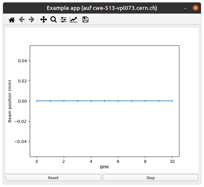
And just like that, our optimization problem is ready to be embedded into a GUI application. Here is a very simple one, in just 54 lines of code:

import jpype
from matplotlib.backends.qt_compat import QtWidgets
from matplotlib.backends.backend_qt5agg import (
    FigureCanvasQTAgg as FigureCanvas,
    NavigationToolbar2QT as NavigationToolbar,
)
from pyjapc import PyJapc
from coi_example import AwakeElectronBeamSteering
# Requires `pip install cernml-coi-utils`.
from cernml.mpl_utils import iter_matplotlib_figures

class MainWindow(QtWidgets.QMainWindow):
    def __init__(self) -> None:
        super().__init__()
        japc = PyJapc("", noSet=True, incaAcceleratorName="AWAKE")
        self.problem = AwakeElectronBeamSteering(
            japc=japc,
            render_mode="matplotlib_figures",
        )
        self.x_0 = self.problem.get_initial_params()
        figures = self.problem.render()
        # We assume just a single figure.
        for _, figure in iter_matplotlib_figures(figures):
          self.canvas = FigureCanvas(figure)
        reset = QtWidgets.QPushButton("Reset", clicked=self.on_reset)
        step = QtWidgets.QPushButton("Step", clicked=self.on_step)
        widget = QtWidgets.QWidget()
        self.setWindowTitle("Example app")
        self.setCentralWidget(widget)
        self.addToolBar(NavigationToolbar(self.canvas, self))
        buttons = QtWidgets.QHBoxLayout()
        buttons.addWidget(reset)
        buttons.addWidget(step)
        layout = QtWidgets.QVBoxLayout(widget)
        layout.addWidget(self.canvas)
        layout.addLayout(buttons)

    def on_reset(self) -> None:
        self.problem.compute_single_objective(self.x_0)
        self.problem.render()
        self.canvas.draw_idle()

    def on_step(self) -> None:
        params = self.problem.optimization_space.sample()
        self.problem.compute_single_objective(params)
        self.problem.render()
        self.canvas.draw_idle()

def main():
    app = QtWidgets.QApplication([])
    window = MainWindow()
    window.show()
    app.exec_()
    jpype.JPackage("java").lang.Thread.detach()

if __name__ == "__main__":
    main()